Linear Regression in machine learning (with example)
Table of Contents
Linear Regression is a great starting point for beginners in Machine Learning and can be used as a base model to compare other more complex algorithms.
What is Linear Regression?
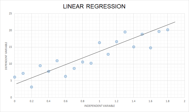
Regression in statistics is a technique that models the relation between the dependent variable to one or more independent variables.
“Linear Regression attempts to approach the regression technique using linear equations”
Let us go through the steps involved in the Linear regression algorithm using a detailed example.
Example (Step-by-Step)
Simon is a star employee of a brokerage firm. He has been assigned following task by his boss.
Task: The company gets a quotation of 380,000 $ for a house of 2000 feet^2. Should the company close the deal or not?
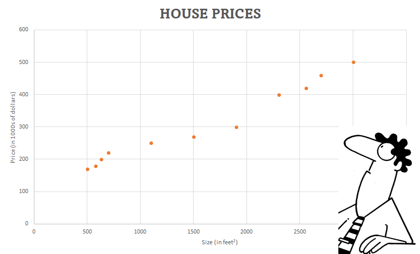
To start with, Simon takes a look at the company’s past database and plots the prices for which the company got the deal for different sizes of houses. Luckily, he observed a linear relationship between the data points. And so, he decides to use the Linear Regression technique.
Now, let us go step by step into it.
Step 1: Model Representation
The first step is to create a model that will be used to predict the price of the house. As Simon knows that the model has to be linear in nature, he decides to use the general line equation.
h_{\theta}(x) = \theta_0 + \theta_1 x
where,
\theta_0, \theta_1: Parameters of the model to be determined x : Input/ independent variable (Size of the house) h_{\theta}(x): Predicted output/ dependent variable (Predicted price)
Since the model has just one dependent variable, this method is also known as univariate linear regression.
Step 2: Cost Function
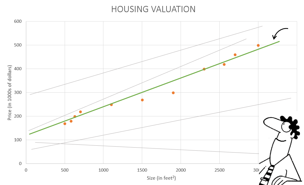
In the second step, Simon has to optimize the parameters \theta_0, \theta_1 such that the model predicts the values closest to the actual output data. Accordingly, he uses a cost function : J(\theta_0,\theta_1)
“A cost function determines how well a machine learning model performs on a dataset”
In the function, h_{\theta}(x^i)-y^i represents the error when comparing predicted output with the correct output of the i-th entry of the data.
Further, the error term is squared since we are only concerned with the distance between the predicted outputs and correct outputs, irrespective of their sign. (Of course, there are other ways to define the error function, but this is the most common function in linear regression algorithms)
Then, the error is summed together for m training examples. And finally, it is divided by 2m , to ensure that the cost function is not dependent on the number of training examples.
Overall, the above cost function gives an estimate of the total normalized deviation or error in the prediction with respect to the correct values. And this error needs to be optimized.
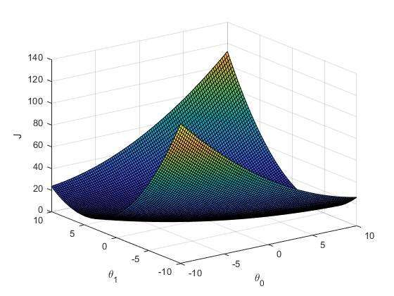
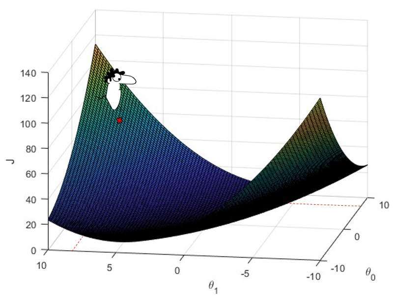
Below you can visualize the cost function for different values of \theta_0, \theta_1.
There is a point on the surface where Simon’s cost function has minimum value. And, in order to find the best fitting line of the data, the minimum point of the cost function needs to be known.
Since Simon can’t take the headache of calculating the cost function at all possible values and then compare each and every value for minima. Therefore, he chose to use Gradient descent algorithm.
“Gradient descent is a first-order iterative optimization algorithm for finding a local minimum of a differentiable function”
But how it works ???
Let us say, that Simon starts with some random values of \theta_0 and \theta_1 . This point is marked on the cost function surface plot below.
Now, I want you to imagine it as a landscape where he is standing at the start point. And he knows that he has to go to the lowest point but he can’t see the whole landscape at once (Although in our case the cost function is very simple). So he turns around and looks for the steepest downhill around him. This steepest downhill can be formulated as the gradient of the cost function at the start point \theta_0^0 and \theta_1^0 .
Gradient: \frac{\partial J(\theta_0^0,\theta_1^0)}{\partial \theta_j} (for j=0 and j=1)
You can see now why the squared error cost function has ‘2’ in the denominator (as it cancels out in the gradient term).
Based on the calculated gradient, he can simultaneously update the values of \theta_0^0 and \theta_1^0 , to reach a new point \theta_0^1, \theta_1^1 using below formula –
where \alpha is the learning rate and represents the step size in the exact opposite direction of calculated gradients (that’s why the negative sign).
Further, he repeats the above steps until convergence of \theta_0 and \theta_1 to get optimal parameters.
Step 4: Solving the task
Remember the task to be solved..
Task: The company gets a quotation of 380,000 $ for a house of 2000 feet^2. Should the company close the deal or not?
Simon uses his optimised Linear regression model to predict the house price for an area of 2000 feet^2. The model predicts the price to be around 357,300 $, which is much less than their quotation value. In other words, their company is getting a deal at much better price than the predicted price of the model. So, he immediately calls his boss to close the deal and approve the quotation.
Points to remember
Great!! You almost made it till the end. Now since you know how the Linear regression algorithm works, you must know few basic assumptions that needs to be fulfilled to mark the success of the algorithm.
First of all, there must be a linear relationship between the dependent and independent variables.
The observations (house prices in our case) should be independent of each other.
There must not be any outliers (data point which differs significantly from other observations) in the data.
Summary
In summary, the blog aimed to provide a comprehensive overview of the Linear Regression algorithm. From understanding the basic concept to its implementation, we have covered all the important aspects.
I hope you find the blog informative and useful. Now, I encourage you to try implementing the concepts discussed in this blog to your own projects. Further, if you want to have an hands-on introduction to ML pipeline in python, refer my other blog here.
Thank you for reading the blog.
Share:
8 Responses
Normally I do not read article on blogs however I would like to say that this writeup very forced me to try and do so Your writing style has been amazed me Thanks quite great post
Attractive section of content I just stumbled upon your blog and in accession capital to assert that I get actually enjoyed account your blog posts Anyway I will be subscribing to your augment and even I achievement you access consistently fast
I simply could not leave your website without expressing my admiration for the consistent information you provide in your visitors. I anticipate returning frequently to peruse your new postings.
Great post. I was checking constantly this weblog and I’m inspired! Extremely useful information specially the closing part 🙂 I take care of such info a lot. I was looking for this particular information for a long time. Thank you and best of luck.
Logistic regression is a machine learning model that helps in the classification of the data in pre-defined classes. The classification can be either binary (two-class)
Generative Adversarial Networks (GANs) are popular for their capabilities in generating fake data, including fake images or videos. But what made them so powerful? Read to know more about their architecture and training process.
In machine learning, a pipeline is a sequence of automated data processing and modeling steps that convert raw data into a refined predictive model. Read this blog to get hands-on tutorial on end-to-end development of a pipeline using Python.
ChatGPT is the single fastest growing human application in the whole history. It had around 100 million users in just 2.5 months from its launch date. What exactly is about ChatGPT that made it widely popular?


8 Responses
Normally I do not read article on blogs however I would like to say that this writeup very forced me to try and do so Your writing style has been amazed me Thanks quite great post
Thank you !
Attractive section of content I just stumbled upon your blog and in accession capital to assert that I get actually enjoyed account your blog posts Anyway I will be subscribing to your augment and even I achievement you access consistently fast
Glad that you enjoyed. Thanks
I simply could not leave your website without expressing my admiration for the consistent information you provide in your visitors. I anticipate returning frequently to peruse your new postings.
Thank you for your kind words.
Great post. I was checking constantly this weblog and I’m inspired! Extremely useful information specially the closing part 🙂 I take care of such info a lot. I was looking for this particular information for a long time. Thank you and best of luck.
Thank you!