Logistic regression is a machine learning model that helps in the classification of the data in pre-defined classes. The classification can be either binary (two-class) classification, or multinomial (multiple-class) classification.
In real world scenarios, examples of binary classification can be classifying an email as spam or not spam, or diagnosing a patient with cancer or not cancer. While, multinomial classification tasks could be classifying images into numbers or text, for instance classifying the famous MNIST dataset.
If you are a complete beginner and want to have a quick introduction to the classification tasks in machine learning before moving on to implementation part. Then I would recommend reading this short blog on “Classification in Machine Learning: A Brief Introduction“
If you are ready, then let’s roll up our sleeves for some hands-on work with Python.
The Classification problem
In this tutorial, we have covered the popular Python library called scikit-learn (aka sklearn). This library contains simple and efficient tools for predictive data analysis, including classification and regression models. For the scope of this blog, we would be discussing the logistic regression model for a given classification problem.
The dataset for our classification problem is cited from Cortez et al., 2009. It consists of the wine (red+white) quality data of the Portugese “Vinho Verde” wine. These wines are loved for their mouth-zapping acidity, subtle carbonation, and lower alcohol – making them a great choice for summer.
Our task is to train a logistic regression model that classifies them as good or bad quality wines based on given input features. However, for simplification we have only considered the red variant of the wine quality data. Also, due to privacy and logistic issues, only physicochemical (inputs) and sensory (output) variables are available. For instance, unfortunately, there is no data about the brand of the wine, the types of grapes, or the selling price.
This section will cover step-by-step tutorial on logistic regression using Python.
Let us start by importing the required libraries.
					import numpy as np # linear algebra
import pandas as pd # data processing
import seaborn as sns # data visualization
from sklearn.linear_model import LogisticRegression #LR model
1) Loading the dataset
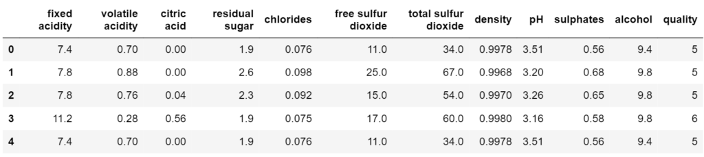
Once the dataset is downloaded and saved in the same directory, the csv file can be loaded in the environment using pandas ‘.read_csv’ method.
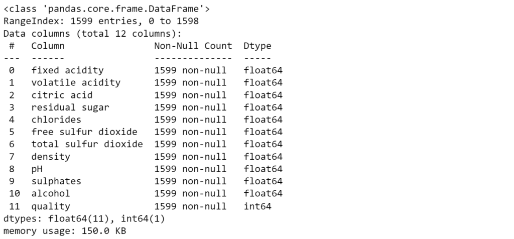
As we can see, the dataset contains 12 columns with quality as the output feature that the model needs to predict. Further, to know more about the type of data and the number of data entries, we can use the following methods from pandas.
wine.info()
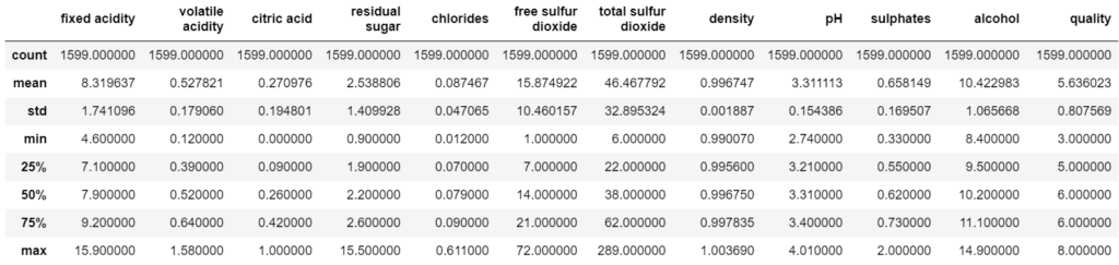
wine.describe()
In total, we have 1599 non-null entries. Also, the ‘quality’ column ranges from minimum value of 3 to maximum value of 8. So, to transform the continuous data to categorical values, we need to threshold the quality values. In our case, values greater than or equal to 7 are considered good quality wines while less than 7 are considered bad quality wines.
2) Data pre-processing
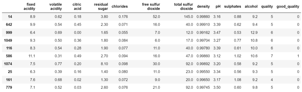
Based on thresholding, a new column ‘good_quality’ is created in the dataset with values 0 and 1 for bad and good quality respectively.
					#setting the wine quality between 1 and 0, if wine quality is >=7 is good which means 1
wine['good_quality'] = [1 if x >= 7 else 0 for x in wine['quality']]
wine.sample(10)
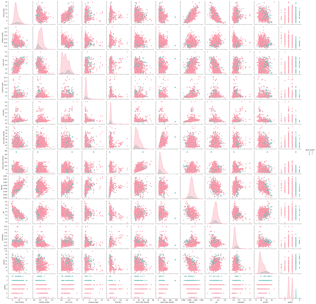
The above figure shows the correlation between the features. For instance, ‘fixed acidity’ and ‘pH’ values are negatively correlated, as expected. That means, as the ‘fixed acidity’ of the wine rises, the ‘pH’ value decreases. Also, the points are plotted based on the values of ‘good_quality’ data in green and red colored points respectively.
import matplotlib.pyplot as plt
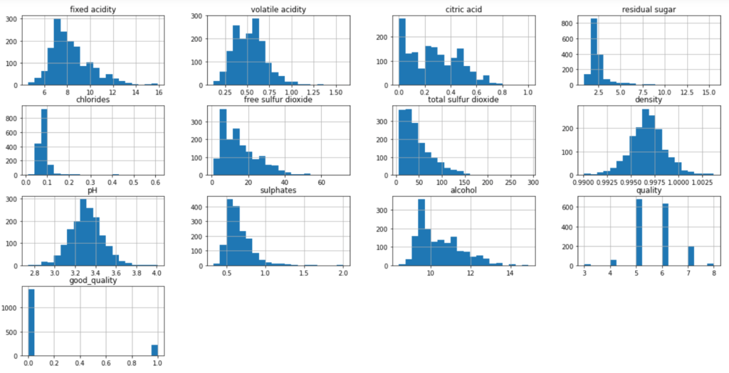
wine.hist(bins=20, figsize=(20, 10)) #bins =40
plt.show()
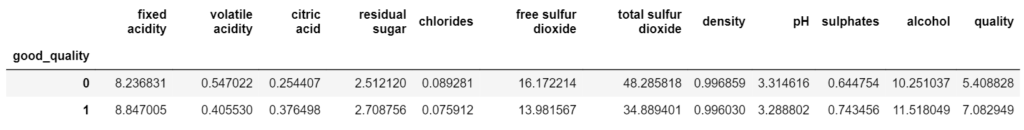
wine.groupby('good_quality').mean()
Once the data is processed, we can see the characteristics of good quality Portugese wine. For instance, as per the above table, good quality wines have lesser content of free sulfur dioxide and higher alcohol content.
Now, we are ready to train our model on the dataset.
3) Preparing the dataset
					X = wine.copy()
y = X['good_quality']
X = X.drop(['quality','good_quality'], axis =1 )
In order to train the model, the dataset is split in training and test dataset. We have kept the ratio as 70:30, where training data contains 70% of the dataset while test data contains 30% of the dataset.
					from sklearn.model_selection import train_test_split

X_train, X_test, y_train, y_test = train_test_split(X_new, y, test_size=0.3, random_state=7)
Further, the random state parameter is passed to reproduce the same results on every run.
4) Fitting the model
Once the data is prepared, an instance of the logistic regression class from sklearn is created with the max_iter parameter set to 2000. This will allow enough iterations for the model to reach an optimum value before the stopping criteria is met.
Further, the model is fitted on the training dataset of our wine quality data.
					model = LogisticRegression(max_iter=2000, verbose =1)
# fitting the model with data
model.fit(X_train, y_train)
5) Measuring performance
In order to measure the performance of our trained model on the test dataset, there are several metrics that can be used. These include the accuracy, F1 score, precision, recall, etc. However, for simplification we use only accuracy score as our performance metrics.
The accuracy score is calculated based on the number of correct predictions on the test dataset.
where, 1(x) is the indicator function which is equal to 1 if the condition inside is true and 0 otherwise.
					# see the classification results
y_pred = model.predict(X_test)
from sklearn.metrics import accuracy_score
print("Accuracy:",accuracy_score(y_test,y_pred))
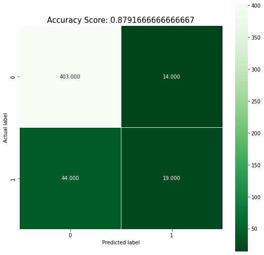
Accuracy: 0.879
The trained model can achieve an accuracy of 87.9% which can be further improved based on the requirements.
Besides the accuracy score, a confusion matrix is also calculated for the model. It can further help investigate the performance based on the matrix. For instance, we can derive the accuracy, precision, recall and F1 score from the table itself.
In our case, as the problem is binary classification, the confusion matrix generated is a 2×2 matrix. Furthermore, we have used seaborn library to visualize the confusion matrix in a visually appealing way.
To learn more on the confusion matrix, refer the sklearn documentation here.
Further Improvements
Up until now, we discussed the available methods in scikit-learn, that allow us to train and test the logistic regression model. Further, if the achieved accuracy is not good enough, we can improve it by either enhancing the dataset or tuning the model for optimum hyperparameters. To do so, there are different techniques that can be employed. Some of them include –
Removing suspected outliers
Normalization/Standardization of the input data
Feature selection
Hyperparameter tuning
If you want to learn more about these techniques, they will be further discussed in the second part of the tutorial video on logistic regression. The video will be uploaded soon on my channel – ThinkUponAI
Summary
In conclusion I would like to mention that training a logistic regression model using sklearn is simple but not always enough. It is equally important to optimize and tune the model parameters in order to achieve the required accuracy.
In summary, we implemented steps including –
loading the dataset using pandas dataframe
thresholding output data for two-class classification problem
splitting the data in training and test data
fitting the logistic regression model
measuring performance using performance metrics
Tips on improving the performance of the model
Hope you learned something from it. As a next step, you can try implementing other classification or regression models from scikit-learn library on the same dataset and compare the results.
Thank you for reading the blog.
Share:
6 Responses
Fantastic site Lots of helpful information here I am sending it to some friends ans additionally sharing in delicious And of course thanks for your effort
Normally I do not read article on blogs however I would like to say that this writeup very forced me to try and do so Your writing style has been amazed me Thanks quite great post
I do trust all the ideas youve presented in your post They are really convincing and will definitely work Nonetheless the posts are too short for newbies May just you please lengthen them a bit from next time Thank you for the post
Logistic regression is a machine learning model that helps in the classification of the data in pre-defined classes. The classification can be either binary (two-class)
Generative Adversarial Networks (GANs) are popular for their capabilities in generating fake data, including fake images or videos. But what made them so powerful? Read to know more about their architecture and training process.
In machine learning, a pipeline is a sequence of automated data processing and modeling steps that convert raw data into a refined predictive model. Read this blog to get hands-on tutorial on end-to-end development of a pipeline using Python.
ChatGPT is the single fastest growing human application in the whole history. It had around 100 million users in just 2.5 months from its launch date. What exactly is about ChatGPT that made it widely popular?


6 Responses
Fantastic site Lots of helpful information here I am sending it to some friends ans additionally sharing in delicious And of course thanks for your effort
Thanks!
Normally I do not read article on blogs however I would like to say that this writeup very forced me to try and do so Your writing style has been amazed me Thanks quite great post
I do trust all the ideas youve presented in your post They are really convincing and will definitely work Nonetheless the posts are too short for newbies May just you please lengthen them a bit from next time Thank you for the post
Sure. Will consider your feedback next time.